Transformers for Node Classification

[zak_jost]

This post is an experiment in doing open research. It’s unclear what general value it will offer, if any. The plan will be to document my thinking and progress as they develop. Comments/questions are encouraged.

Motivation

In practice, many real-world graphs of interest evolve in time. For example, graphs representing users and their connections for purposes of fraud detection, or their interactions with products for recommendation systems, both have a constant stream of new nodes and edges, and potentially dynamic features that change in time. This presents at least 4 distinct problems for traditional GNNs:

1. The majority of GNN methods in the literature are transductive, meaning they do not generalize to unseen nodes/edges. This is an egregious problem because it’s often the new items that are of particular interest and in need of a prediction. In practice, these methods need to be retrained when the graph changes, and this presents a number of operational problems. We therefore need an inductive model to be useful in most practical applications.
2. Most GNN methods assume a static graph and have no capability to leverage temporal information. Temporal information is key in many problems, however. For example, a rapidly emerging cluster of users is perhaps more suspicious in fraud applications, or predictive of a viral/timely piece of content in a recommendation context.
3. Popular GNN modeling frameworks, like Deep Graph Library and PyTorch Geometric, were not designed to elegantly handle time-evolving graph data structures, features, or time-aware message-passing operations. As a result, implementing time-aware models is often difficult, inefficient, or reliant on approximation schemes, like treating the graph as a series of static snapshots that trade-off memory with approximation quality. Simple mechanisms like edge masking can be employed for dynamic edges, but handling evolving features presents additional complications.
4. The static graph assumption (and the frameworks built on this) causes yet another problem: message passing operations themselves are not time-aware and as a result, models often leak information from the future during training. The models do not have this advantage in a production setting, of course, and therefore suffer in performance.
   • As an example, in the ogbn-arxiv benchmarks, the graph methods first reverse the edges, meaning that a classification decision for a paper not only depends on what it cites, but also on who cites it in the future. If the goal is to classify new papers, clearly these future citations will not be available and this model’s real-world performance will be far lower than what’s reported on the test set.

In sum, there’s a significant disconnect between existing GNN methods, frameworks and benchmarks, and many real-world industrial problems. As a consequence, many approximations and compromises need to be made.

Hypothesis

My hypothesis is that by sampling a subgraph around a target node, we can use transformers to aggregate this information into a prediction that more naturally models the problem, particularly for dynamic graphs. Instead of having a large graph structure that’s used for message passing, we instead pre-process our data to construct a collection of subgraphs. These choices give us a number of benefits:

• The model is trained on localized subgraphs and is therefore naturally inductive, and will generalize to new subgraphs.
• Temporal information can be naturally represented via temporal encodings of the entities, allowing the model to leverage temporal dynamics without significant incremental effort.
• There exists a large community investment in transformer tooling and this method removes the need to rely on the complexities of GNN training and frameworks, like handling message passing in distributed training environments. This approach can be trivially parallelized.
• Since we do not need a single representation of connection structure, each neighborhood snapshot can be point-in-time correct relative to the target node. This removes the need to have in-memory data structures that can elegantly handle all the time-evolving information and prevents future information leakage. Unlike in GNNs, this allows us to, for example, easily include neighbor labels as features.
  • GNNs need to resort to various tricks to handle this use case of “labels as features”, like stochastically removing label features during training. See the Label Usage section here for an example.

Challenges

The key challenge here is figuring out how to usefully encode graph structure so that the transformer can make efficient use of it. There are a few ideas:

• Use an approach similar to Pure Transformers are Powerful Graph Learners, which encodes a graph structure by concatenating positional representations of the source/destination pairs of nodes that have edges: \{ P_u \Vert P_v : (u, v) \in \mathcal E \}, where the P_i positional encodings are just required to be orthonormal.
• Learn graph-aware node encodings based on things like:
  • Shortest path length from the target node
  • Node type, or shortest meta-path to target node, for heterogeneous graphs
  • A structural property of the nodes, like degree, or “color” resulting from running the W-L algorithm
  • Some combination of the above

[zak_jost]

OGBN-ARXIV baseline

To develop the code and intuition, I will start with a simple node classification benchmark, for which there are many available implementations: ogbn-arxiv. This represents a citation graph where the nodes are papers and the edges are citations. Nodes come with features that represent word embeddings of the title/abstract. The task is to classify a node as belonging to 1 of 40 possible topics.

My goal is to beat a simple baseline GNN method, like GraphSAGE.

Relevant baselines (validation accuracy, test accuracy):

• MLP: (0.5765 ± 0.0012, 0.5550 ± 0.0023)
• Label Propagation: (0.7014 ± 0.0000, 0.6832 ± 0.0000)
  • reversed edges
• GraphSAGE: (0.7277 ± 0.0016, 0.7149 ± 0.0027)
  • reversed edges
  • 3 GNN layers

[zak_jost]

A few notes on the baselines. As mentioned in the first post, the models on the leaderboard reverse the edges in the graph before building models, which effectively means that a classification decision for a paper not only uses information from the papers it cites, but also the future information from the papers that end up citing the target paper. This turns out to strongly influence the results for baseline GNN methods.

The following are the validation/test results of a single run of the leaderboard’s GraphSAGE model, but without reversed edges and evaluated using different numbers of layers/hops:

• Leaderboard settings (3-hop): (0.6406, 0.5674)
• 2-hop: (0.6318, 0.5675)
• 1-hop: (0.6197, 0.5594)

While the number of hops seems to not make much of a difference, note that there is an enormous performance drop from 71.5% down to 56.7%. At this point, it’s unclear what drives this performance gain, exactly.

Parenthetically, I think this is a mistake and should be forbidden in the benchmarks, because we presumably would use the model for classifying new papers, which have not yet been cited and the evaluation will obfuscate performance in this setting since most papers in the test set have citations. Regardless, I will also reverse edges in my future experiments so that I can compare apples-to-apples, but ultimately hope to revisit this without reversed edges so that we can better understand generalization ability.

[zak_jost]

Simple models

My first experiments will be aimed at understanding how simple alternatives to GNNs compare. I start with two models:

• SAGESim: this is similar to GraphSAGE in that it applies a linear layer to neighbors’ features, averages the results, and adds the result: h = W_0*x_0 + W_1 \text{avg}(\{x_1\}) + W_2 \text{avg}(\{x_2\}), where \{x_k\} represents the word vectors of the k-hop neighborhood of the target. The intuition is that the separate linear layers for each hop will learn to appropriately weight information coming from this graph distance. The only difference with GraphSAGE is that the average is taken of the raw features, rather than updating iteratively as in GNNs, such that the 2-hop features are used to calculate 1-hop embeddings, which are then used to calculate target embeddings.
• MHA: a multi-head self-attention layer that operates directly on the multi-set of neighbors. Positional encodings are indexed by the shortest path length of the node to the target. E.g., the target node has index of 0, 1-hop neighbors an index of 1…etc, and then embeddings are learned for these positions and added to the raw features. The output embedding of the target node is then extracted and passed through a linear layer to make a final prediction.
  • Note that in principle, this model could learn to re-create SAGESim if the MHA process effectively averaged item features that had the same positional encoding.

Neighbor sampling

For my models I sample up to 100 1-hop neighbors, and 1 2-hop neighbor for each 1-hop, giving a total of up to 200 possible neighbors. This is done in a single pre-processing step, so each target node always has the same sampled neighbors. No neighbor sampling was done for the baseline GNN methods.

Results

The following use reversed edges on the graph.

1-hop neighborhood

• SAGE 1-hop: (0.6774, 0.6650)
• SAGESim 1-hop: (0.6824, 0.6710)

2-hop neighborhood

• SAGE 2-hop: (0.7202, 0.7092)
• SAGESim 2-hop: (0.6895, 0.6802)
• MHA: (0.6971, 0.6909)

While it was straight-forward to exceed peformance in the 1-hop setting, I was not able to get SAGESim or MHA to meet or exceed performance in the 2-hop setting despite many efforts.

[zak_jost]

Today, I will focus on understanding how GNNs get benefit from 2-hop information.

First, I will focus on pre-computing neighborhood averages and replacing the features. I.e., each node feature is replaced with the average of its direct neighbors. This effectively pre-computes the first GNN layer, and then I’m left with simulating the last layer. This can be expressed as X_\text{avg} = \alpha \hat A^k X + (1-\alpha) X, where \hat A is the row-normalized adjacency matrix.

The SAGESim should be able to exactly recreate GNN performance. If not, there’s something I am missing. Assuming that pans out, I can hopefully get similar (or better!) results with the xformer.

Experiments

• SAGESim with 1-hop neighbors, using A*X features for all nodes: (0.7106, 0.7026)
  • Since the first neighborhood aggregation was pre-computed, this is similar to learning the last GraphSAGE layer.
  • This effectively matches performance on the test set.
• MHA
  • 2-hop, using A*X for all nodes: (0.7148, 0.7076)
  • 1-hop, using A*X for all nodes: (0.7127, 0.7053)
  • 1-hop, using A^2*X for all nodes: (0.7165, 0.7093)
  • 1-hop, using A^3*X for all nodes: (0.7205, 0.7081)
  • 1-hop, using A^3*X with alpha=0.2 for all nodes: (0.7209, 0.7112)
  • 1-hop, using A*X for 1-hop, original features for target: (0.7140, 0.7046)
  • 1-hop, A^2*X for 1-hop, original for target: (0.7192, 0.7127)
  • 1-hop, A^3*X for 1-hop, original for target: (0.7185, 0.7107)
  • 1-hop, A^3*X with alpha=0.2 for 1-hop, original for target: (0.7210, 0.7162)

Take-aways

• This closes the gap and allows MHA to exceed performance of GNNs. It seems that smoothing of the neighbor features is key. This may suggest there’s too much noise/variance in individual paper’s word embeddings
• Retaining the original feature of the target node seems to be helpful, but can overfit.

Follow-up ideas

What do I do with the knowledge that this sort of feature-smoothing seems to be important? Try message passing on the subgraph to locally smooth the features. I.e., for a given subgraph A_sg, smooth the features X before passing into the transformer: y = MHA(A_sg^k*X)

[zak_jost]

We last found that smoothing the features via feature propagation improved performance of a multi-headed attention (MHA) layer compared to operating directly on the raw features. By doing this, the MHA model was able to finally match/exceed performance of the GNN.

This begs the question: are other types of smoothing that do not rely on graph structure equally as effective? Here, we test whether it’s effective to replace a paper’s features with the average of itself with its k-nearest neighbors (k-NN).

Experiments

• 2-hop, 10-NN features for all nodes: (0.6961, 0.6891)
  • Seems to be about the same as having no smoothing
• 2-hop, 10-NN features for neighbors, original for target: (0.6966, 0.6871)
• 1-hop, 10-NN features for all nodes: (0.6854, 0.6775)
• 1-hop, 10-NN features for neighbors, original for target: (0.6837, 0.6760)
• 2-hop, 100-NN features for all nodes: (0.6935, 0.6861)
• 2-hop, 100-NN features for neighbors, original for target: (0.6937, 0.6837)

Thinking through implications

This doesn’t work. It makes sense that nearest neighbor smoothing would not work as well as graph smoothing because in the case of the graph, it’s telling you which other nodes are relevant–e.g., the papers I’m citing are particularly relevant. For NN-smoothing, it’s simply reducing variance. It begs the question: is it more predictive of the label to have the same word features, or to be cited?

I still don’t really understand why graph-based smoothing as a preprocessing step helps so much. Is it that the average of the citation network provides a better representation of the label than any particular paper? That seems clear–a logistic regression trained on neighbor averages would outperform one trained on individual node features. I suppose it’s not about variance reduction, per se, but rather about collapsing irrelevant variance by averaging it out, and keeping the essential information. Or, put another way, we make the assumption that two papers that cite many of the same papers have the same label, and we give them similar representations by averaging together the features of all the citations.

Follow-ups

• Answer: Do papers tend to have the same labels as those they cite? Do nearest neighbors of features tend to have the same label?
  • Papers tend to have the same label as those they cite with a median accuracy of 71% of 1-hop neighbors. NNs do not tend to have the same labels, with a median accuracy of 100-NNs at 27%.

[zak_jost]

Smoothing the features via averaging with nearest neighbors did not seem to work well. What if we apply feature smoothing on the induced subgraph after sampling the k-hop neighborhood of a target node? I.e., sample a neighborhood and create the (row-normalized) adjacency of the subgraph, \hat A_{sg}, and then calculate smoothed features via: X_\text{avg} = \alpha \hat A_{sg}^k X + (1-\alpha) X.

Results

• 2-hop, k=2, input_dropout=0.1: (0.6885, 0.6784)
• 1-hop, k=2: (0.6883, 0.6816)
• 1-hop, k=2, input_dropout=0.1: (0.6868, 0.6759)
• 1-hop, k=2, input_dropout=0.3: (0.6884, 0.6791)

take-aways

This does not work.

UPDATE: this may not be a proper test due to the way I sampled. In particular, since I’m sampling 100 1-hop, but 1 2-hop for each 1-hop, this means the 1-hop neighbors are all averaging together itself with a single one of its neighbors, which likely won’t have a significant impact. We might instead try this on a fanout like (25, 25).

[zak_jost]

One of the key advantages of using a transformer is the ability to create point-in-time correct features for the target node. In this case, it allows us to use the labels as features for our neighbors, effectively utilizing something like Label Propagation in the attention mechanism.

In particular, we one-hot encode (OHE) the 40 possible labels for each of the neighbors, and concatenate this encoding to the raw paper text embeddings. Care is taken to make sure that the label of the target node is not included as a feature, even if the target node is sampled as part of the 2-hop neighborhood. The target label is overwritten with a dummy and is given a special column in the OHE.

• 2-hop, seq of OHE labels, dropout=0.1: (0.7497, 0.7381)
• 2-hop, seq of OHE labels, dropout=0.2: (0.7507, 0.7379)
• 2-hop, seq of OHE labels, exclude_words=True, dropout=0.1: (0.7336, 0.7205)
  • This only uses the OHE labels and ignores the word embeddings.
• 1-hop, seq of OHE labels, dropout=0.2: (0.7476, 0.7379)
• 1-hop, seq of OHE labels, input_dropout=0.1, MHA dropout=0.1: (0.7465, 0.7357)

Take-aways

This greatly exceeds performance of GraphSAGE baseline and puts the method in the top 30 on the leaderboard.

Follow up: what are the failures exactly? Manually look at some to understand. Are they ones with a large number of neighbors, but of different label? No neighbors? Mistaken labels?

[zak_jost]

Now that I have the basics worked out, I’d like to implement the transformer and verify it at least matches the MHA performance.

• 2-hop, num_layers=1, input_dropout=0.1: (0.7505, 0.7379)
• 2-hop, num_layers=1, input_dropout=0.2: (0.7497, 0.7379)
• 2-hop, num_layers=1, input_dropout=0.2, mha_dropout=0.1: (0.7515, 0.7358)
• 2-hop, num_layers=2, input_dropout=0.2, mha_dropout=0.1: (0.7502, 0.7356)
• 2-hop, num_layers=5, input_dropout=0.2, mha_dropout=0.2: (0.7489, 0.7398)
• 2-hop, num_layers=5, input_dropout=0.2, mha_dropout=0.5: (0.7511, 0.7382)
• 2-hop, num_layers=5, input_dropout=0.3, mha_dropout=0.1: (0.7518, 0.7334)

Take-away

Matches and slightly exceeds. This suggests there may be value in adding model complexity, but not much.

[zak_jost]

Next, I want to add the graph-smoothed features to the OHE label features and see if this gives additional performance gains.

Experiments

Using the feature-smoothing that previously gave the best results, which corresponds to X_avg = 0.8*A^3*X + 0.2*X for the neighbors, and raw features for the target.

• 2-hop, num_layers=5, input_dropout=0.2, mha_dropout=0.2: (0.7507, 0.7329)
• 2-hop, num_layers=1, input_dropout=0.1: (0.7513, 0.7353)

Take-aways and interpretations

Smoothing the features in this way did not seem to benefit performance. My hypothesis is that these smoothed features effectively became vectors that mapped to the labels–it’s the job of the first GNN layers to do this smoothing and the job of the last linear layer to learn this mapping. This is more effective than providing raw features of neighbors as a set because it’s a harder task for the model to have to learn how to selectively aggregate these features, and then map to labels, because it needs to deal with the variance presented by each individual paper.

However, when the neighbor labels are directly provided, there is no need to learn these intermediate smoothed vectors. This is likely why performance was so strong for the case where no word vectors were used at all, and only the OHE of neighbor labels was used as features, which obtained performance of (0.7336, 0.7205). I suspect performance is only degraded here because there are cases with no/few neighbors, and the word embedding of these is sufficient to provide a reasonable prediction, as a simple MLP on the raw features demonstrates.

Follow-up

Do an analysis on the failure cases when only the neighbor labels are used, and confirm the hypothesis that performance is only meaningfully worse on those papers with little-to-no neighbors.

[zak_jost]

Note: it seems it was clarified in a GitHub issue that labels of the validation/test nodes cannot be used as features. While my results take care to not leak the label of the target, the validation/test labels are not removed. I will need to re-run to measure the impact of this constraint, but point out this is a synthetic limitation that would not apply in a real-life setting, and is mainly an artifact of being careless by allowing reversed edges.

[zak_jost]

I re-ran experiments using the Multi-headed Attention model with validation/test labels overwritten with dummy values and observed the following:

• MHA, input_dropout=0.1: (0.7173, 0.7008)
• MHA, input_dropout=0.2: (0.7195, 0.7056)
• MHA, input_dropout=0.5: (0.7220, 0.7077)

Overall, excluding validation/test labels of neighbors represents a drop in performance from 0.7381 to 0.7077. I also note that increasing dropout on the input features improved performance. I suspect this is because it helps reduce distributional shift between training and evaluation as a consequence of evaluation papers likely having fewer non-null labels in their neighborhoods since, by construction, all papers that cite them occur in the future and therefore also have null labels.

In sum, not using validation/test labels kills performance, but in my judgment is 1/ an arbitrary restriction that does not exist in real life settings and 2/ only presents an information leak problem because of the choice to allow reversed edges.

Moving forward, I will plan to ignore this restriction, and, if there’s time, enforce the “no reversed edges” rule to better understanding generalization ability of these various methods.

[zak_jost]

Deep diving failures of label-only models

I was curious what was causing failures on the ~30% of samples. My previous hypothesis is this represented nodes with little-to-no neighbors and therefore little label information.

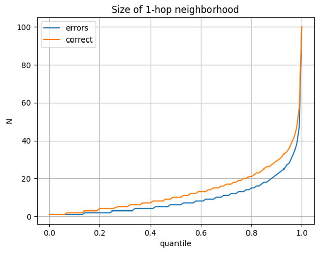
Below plots the percentiles of the 1-hop neighborhood sizes of test nodes that received a correct prediction (orange), or an incorrect prediction (blue).

While the distributions are significantly different, it’s not the case that most of the error cases have almost no neighbors.

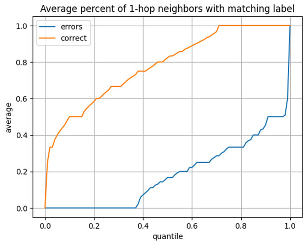
This must mean that the neighbors exist, but are not representative. Next, I plot the quantiles of the percentage of the neighbors that have the same label as the target:

Here we see that for correct predictions, 80% of the neighbors in a neighborhood have the same label as the target node in median, compared to about 17% for incorrect predictions. Or, put another way, the papers that have incorrect predictions tend to cite, or be cited by, papers from different categories than themselves.

For example, the paper “Simultaneous merging multiple grid maps using the robust motion averaging” has category cs.AI. Browsing arXiv’s Bibliographic Explorer tool, only one of the (many) references is on arXiv and therefore included in the dataset, and it’s category is cs.GR (Computer Graphics). Three papers cite the target paper in the relevant time period and are also included as neighbors due to the reversed edges, and they are in the categories: cs.RO (Robotics), cs.NI (Networking and Internet Architecture), and cs.CV (Computer Vision).

The model predicts this is a cs.RO (Robotics) paper, and it’s worth nothing that arXiv does list this as a secondary topic for the paper.

My take-away is that this is a complex task and if this example is representative, it’s no wonder the error rate is high. In this particular case, the word “robot” or “robotics” is used 4 times in the abstract alone, and it cites a robotics paper, so it’s no surprise the model predicted this belongs to the robotics class rather than the AI class.

[zak_jost]

Removing reversed edges

How do various methods compare if evaluated in this more realistic setting?

• SAGE (leaderboard settings): (0.6380, 0.5728)
• MHA on raw features, n_hops=2, input_dropout=0.2: (0.6794, 0.6813)
• MHA w/ label features, n_hops=2, input_dropout=0.1: (0.7157, 0.7227)
• Xformer w/ label features, num_layers=1, n_hops=2, input_dropout=0.1: (0.7171, 0.7260)

Take-aways

• Performance of SAGE is drastically impacted, and drops from 0.7149 to 0.5728
• Performance of MHA has a relatively modest performance drop:
  • When using only word vectors as features: drop from 0.6909 to 0.6813
  • When including neighbor labels as features, drop from 0.7381 to 0.7227
• Performance of the Xformer is slightly better than MHA-only, but perhaps within natural variation

It seems that GNNs are much more sensitive to the inclusion of reversed edges than the attention-based methods.